With the upcoming election, I found myself thinking about the old NYTimes Needle and, more generally, about how to best represent and communicate probabilities.¹

Note: if you want to see how this looks in the context of the 2024 Presidential election, see here.

We already have many ways to discuss degrees of belief: probabilties, percents,² odds, log-odds, nats, bits, decibans, etc. Why don't we add another to the mix. What if we measure degrees of belief in... degrees.

Specifically, let's use the following transformation:

This mapping has a beautiful mathematical justification, gives rise to beautiful visualizations, beautifully aligns with our existing intuitions and has a beautifully simple approximation. What more could you want.

Mathematical Justification

What gives? Where does this mapping come from? Why do we need another way to describe probabilities.

None of the common ways to measure proabilities are statistically uniform. What do I mean by this? Not all 1% changes in probability mean the same thing. Going from 98% to 99% certainty is a much bigger deal than going from 50% to 51%. It requires more evidence. 99% is more distinguishable from 98% than 51% is from 50%. We intuitively know this, no one says they are 61% certain about something, but people will say they are 99% or 95% certain and expect these to mean different things.

To measure this mathematically, we need to look at the most distinguished mathematical measure of distinguishability: the KL divergence. For two Bernoulli distributions with probabilities $p$ and $p + \delta$, the KL divergence is:

To leading order, this is quadratic in the change $\delta$ and depends inversely on the probability $p$ and its complement $1-p$. If we interpret this as a kind of squared distance, the square root of this gives us the usual Jeffreys prior for the Bernoulli problem:

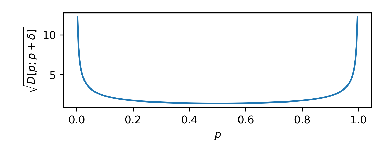
Here we can clearly see that as move towards 0 or 1, the statistical distance blows up. Going from $0.99$ to $0.991$ is 26 times larger a change in terms of KL than going from $0.50$ to $0.501$. Clearly, probabilities measured in percentages are very non-uniform.

If we took as our prior the distribution $1/(\pi\sqrt{p(1-p)})$ we would be weighing the probabilities proportional to this statistical distance. That is, we would be putting equal weight on equally distinguishable probabilities. This is what motivated Jeffreys to make his prior. He wanted a truly non-informative prior. Naively, Laplace suggested a uniform prior as being non-informative. But what does uniform mean? If you start with a uniform prior on percentages, it's very non-uniform when transformed into log-odds. Uniform in log-odds is very non-uniform in terms of percentages. If you start with a uniform prior in percents, you'll get a different posterior than if you start with a uniform prior in log-odds. Clearly, your choice of parameterization is influencing your outcome.

If what we care about is the amount of information you need to modify your beliefs, we should weigh our beliefs in proportion to the amount of evidence they would need to move. This is what led Jeffreys to his prior, in the form we see above. He showed that this is proportional to the square root of the determinant of the Fisher metric. Regardless of your choice of parameterization, if you compute the determinant of the Fisher metric in that parameterization and take its square root, you'll recover Jeffreys prior. It is parameterization independent in this sense.

While Jeffreys found a principled motivation for how to define uniformity in a reparameterization independent way, what we don't have yet is a sense of what a principled parameterization is. Not all parameterizations are created equal. Percentages diverge at the extremes. We should be able to do better.

Let's try a second common parameterization. What if we tried to work in terms of log-odds?

We get KL divergences that take the form:

which has the opposite problem as seen below. There is no divergence at the ends, there is a disappearance.

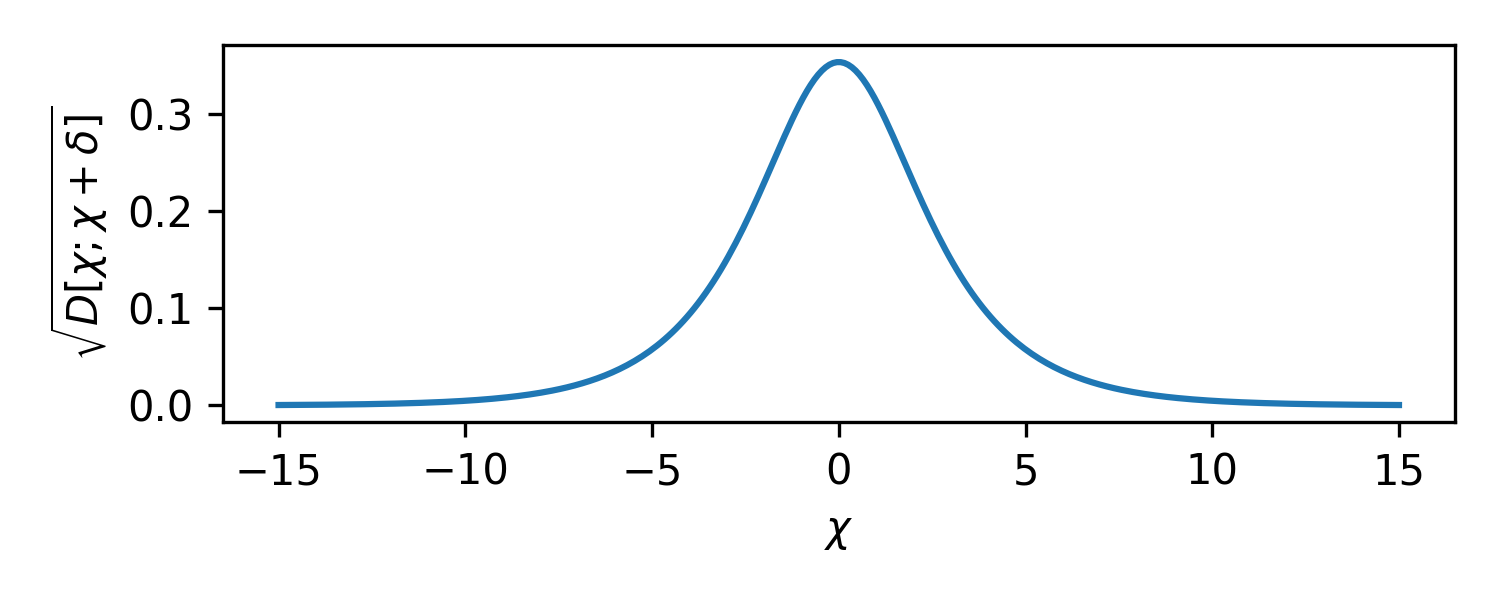
Now, moving from $0.00$ to $0.01$ in log-odds is 42 times farther a statistical distance than going from $5.00$ to $5.01$ in log-odds.³ At the extremes, log-odds become indistinguishable. A log-odds of 7 is closer to 5 than 0.01 is to 0.00.

Very small changes in percentage near 1.0 require massive amounts of evidence to justify. Massive changes in log-odds away from 0 require very little evidence to justify. Neither of these is ideal.

The question then becomes: What is the best parameterization? How close to uniform can we get? Is there a parameterization of degrees of belief for which the statistical metric is flat? Equivalently, the question becomes, is there a parameterization for which Jeffrey's prior is uniform.⁴

Let's look for a transformation, $\theta(p)$, such that, Jeffrey's prior, $p(p) = 1/(\pi\sqrt{p(1-p)})$, transforms into the uniform prior: $p(\theta) = 1$.

Densities transform like:

Substituting what we know, we want to solve:

The solution takes the form (up to proportionality):

This is the mapping we opened the post with. In this parameterization, we have that the KL divergence is flat:

It is in this parameterization that a small change in the parameter means the same thing at every value of the parameter. This parameterization is uniform in a deep sense. Jeffrey's prior, expressed in this $\theta$ parameter is uniform.

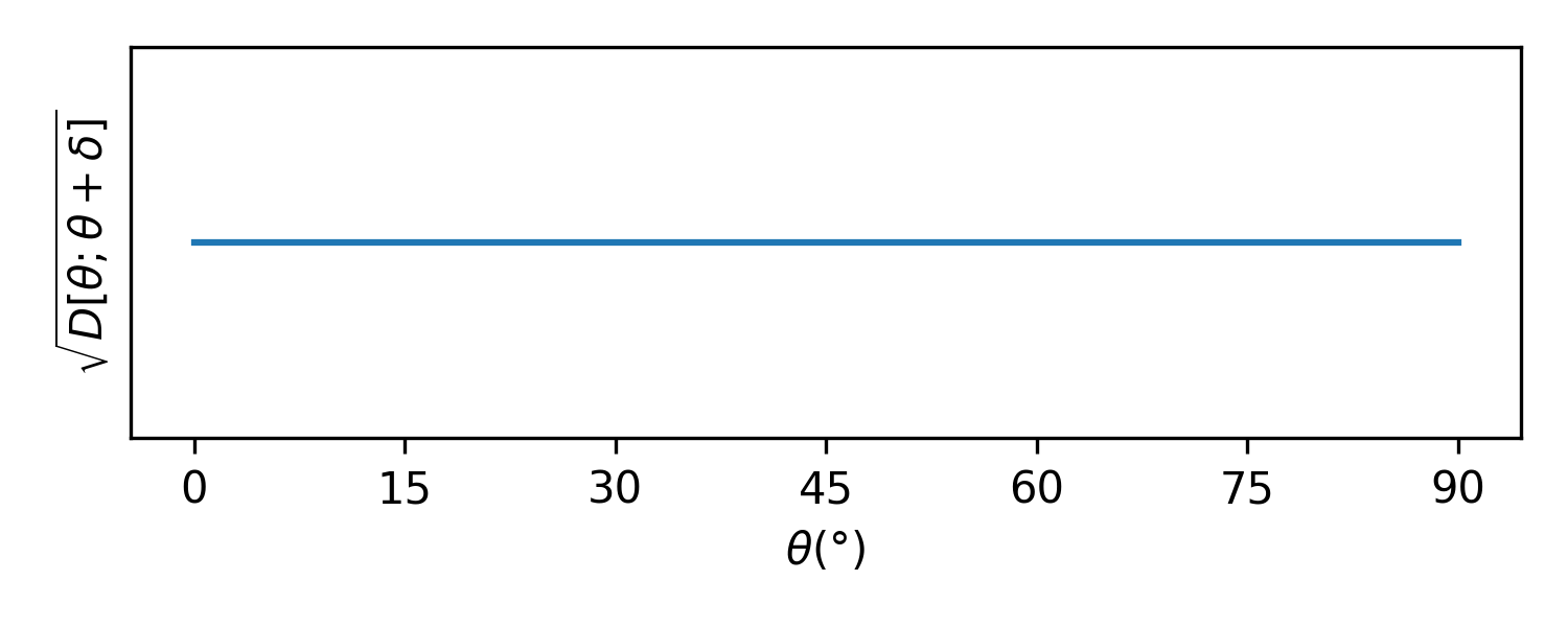
This is, in some sense, the most natural parameterization of probabilities. In terms of ordinary probabilities, the space is curved, the metric isn't flat, the world is distorted as we move around the space. In terms of these degrees ($\theta$), the metric is flat. A 1° change means the same thing, statistically, regardless of where we start.⁵

Visualization

We will set the range of probabilities to be from 0° to 90°. This will allow us to visualize the whole space as a quarter circle, which conveniently resembles a meter when turned on its side.

A probability of 53% corresponds to an angle of 43.28°.

This meter is interactive, you can adjust the probability with the slider or input box.

It turns out that relative angle between two probabilities is related to the Bhattacharyya distance. If we take the straight line chordal distance between two probabilities on this arc, it is equivalent to the Hellinger distance.^6,7

Intuitions

Having identified this mathematically elegant parameterization of degrees of belief, the question remains: is it practical for everyday use?

Well, the more I think about it, the more I think this might actually be a decent idea. People already are familiar with angles and degrees. We have a sense of how large 1° is, or 5° or 30°. We can visualize where these would fall on the meter.

Another benefit of angles is that we already have a strong sense that they are relative.

When probabilities are close to certain, it would be most natural to measure them relative to the right:

For instance, if I say its 10° from certain that Trump will win Texas,⁸ its clear what I mean.

However, we can just as easily measure angles relative to the middle for things that are a toss up:

For instance, we might say that overall, the election is leaning 3.45° in favor of Trump. ⁹

This is clear and easy to visualize and reason about. 3.45° tilted to the right off of vertical is the same as 41.55° out of 90°, but we have a much better intuitive sense of the former. Meanwhile, in terms of percentages, we would say Trump has a 56% chance of winning, we have a much harder time expressing this as a 6% advantage off-even (we might say he has a 12% edge over Harris). This is the whole reason the NYTimes used their needle visualization in the first place. The NYTimes needle provides a useful visual aid, but would be misleading as the probabilities approach 0 or 1, since their linear mapping would distort the changes at the edges. Our nonlinear map maintains a statistical uniformity throughout the whole range.

We could just as easily measure angles with respect to impossibility in the case of rare events:

For instance, we might say there is a 18° chance of Trump winning Virginia:

This versatility comes at no additional mental cost. We already naturally re-orient our discussion of angles in this way. Probabilites and their statistical metric are symmetric about even. Probabilities very near 1 are similar to those very close to 0, but when we talk about percentages, this symmetry is obscured. Log-odds are better in this regard, but much less commonly used.

Kent's Words of Estimative Probability

In the meters on this page, as a visual aid, I've colored six bands of 15° increments. It turns out that these perfectly line up with Kent's words of Estimative Probability.

In an effort to better communicate uncertainty to a lay audience, many people have tried to come up with intuitive names or mappings for different percentages. These always end up corresponding to awkward, unevenly spaced probabilities. For example, Kent, said that 93% corresponds to what people consider "almost certain". 93% seems like a strange value. I always wondered where 93% came form, or why people's intuitions about probabilities were so unevenly spaced. However, if you take Kent's thresholds and map them to degrees, they are perfectly evenly spaced at 15° increments. This suggests that people correct for the statistical unevenness of percentages through experience. The words we use to describe certainty are uniform, even if our most popular unit for measuring certainty is not. This suggests that human perceptions of probabilities might already be better aligned with degrees.

More thoughts on human perception below in Appendix D

Approximate Calculation

While this mapping seems interesting, no one can compute $\arccos \sqrt p$ in their head. Fortunately, as we show below in Appendix A, near the middle the map is linear and near the edges it looks like a square root, so if we want an accurate, easy to calculate, pencil and paper version of the mapping, we can split our probabilities into three regions, below 0.25, between 0.25 and 0.75, and above 0.75.

Since we have that $180/\pi \approx 60$ if we want to estimate the degrees off of even, for a given probability near 50%, in our head we can use: while for $p$ values near the extremes, we can calculate the relative angle you are from either completely certain or impossible as:

If you need a good way to mentally calculate a square root of $p$: take a guess $g$ for the square root, and then compute the average of $g$ and $p/g$. You can iterate this many times to get as accurate as you desire.¹¹

This simple to compute approximate mapping turns out to be very accurate. It is good to half a degree over the whole range as shown below in Figure 6.

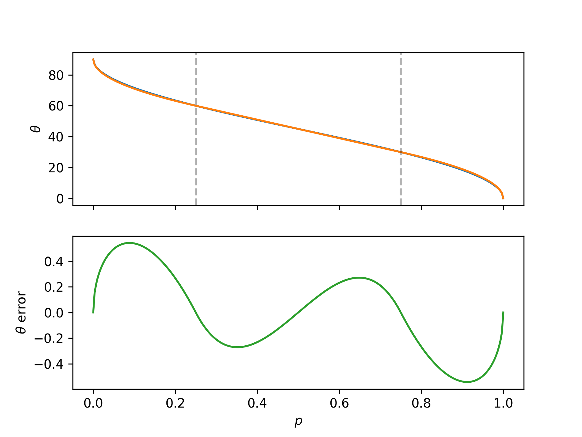
For example, before we said the economist model had Trump's probability of winning at 56%, to estimate this in degrees we take $60 \times 0.06$ to get 3.6°, compared with the more exact 3.45°. If we think there is a 10% chance of rain, we say that that is $60 \times \sqrt{0.10} = 60 \times \sqrt{10} / 10 \approx 19^\circ$, compared with the more exact 18.43°. This method is very practical and very accurate.

Conclusion

I don't know about you, but I'm convinced. We should measure degrees of belief in degrees.

This creates a very intuitive visual representation for probabilities, and one that is statistically uniform in an interesting and useful way. It isn't all that hard to compute, especially if we are alright with a half degree accuracy as in the previous section. With a little bit of time, I think we could come to intuit what a 1° or 5° or 10° or 30° shift in probabilities felt like. Some might even say, we already do. And, unlike with either probabilities or odds, that useful internal sense would work well for us regardless of the baseline rate. A 5° shift away from center means the same sort of thing as a 5° shift away from certainty.

Give a shot. In Appendix C I've made available the code for the widgets that appear on this page, which should make it easy for anyone to try.

Appendix A - Taylor Expansions

If we Taylor expand this map near $p=1/2$, the map is approximately linear:

Near $p=0$ its square root like: And similarly near $p=1$:

Appendix B - Categorical Generalization

This idea easily extends to Categorical distributions, where the flat statistical manifold corresponds to the positive octant of the n-sphere as discussed in Bengtsson et al. ⁶²

Appendix C - Widget

To kickstart its adoption, I've created a WebComponents element, so that you can simply add the script as a module to your page:

<script type="module" src="https://blog.alexalemi.com/assets/Meter.js"></script>

in your <head> section and later insert:

<probability-meter probability="0.53"></probability-meter>

elements to your page and it will render as:

Appendix D - Human Perception

It is generally claimed that human perception aligns well with log-odds. Good¹³ and Jaynes¹⁴ both advocated the use of decibans. These work great for accumulating evidence and doing bayesian updates.

In the field of human perception, I've often seen references to Zhang et al.¹⁵ to justify the claim that human perception is well aligned with log-odds. In the paper they collected a bunch of human perceptual studies and show that you can use a mapping that is linear in log odds to explain the data. For example, here is Figure 1 from the paper:

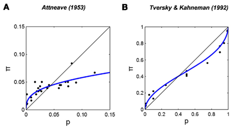
Here, the blue lines show fits of a two parameter function:

which describes a linear map acting on the log odds of the true probability and some baseline probability to describe the log-odds of the perceptual probability. The paper considers it a success that they can use the simple two parameter function to get a mapping that shows good agreement with the experimental data.

You know what these curves look like? They look like our arcsine transformation. Without any parameters, here is a plot of:

This is the same as our proposed mapping (just with the opposite sign).

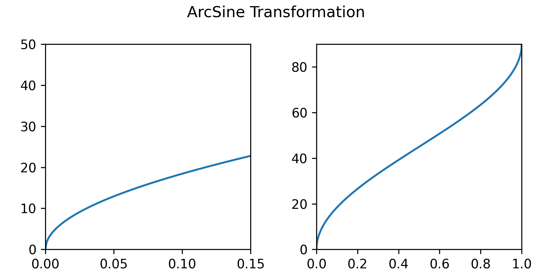
Look's pretty good to me.

Appendix E - ArcSin Transformation

It seems as though there is a history of using the "arcsin" transformation to transform probabilites for statistical models. It seems like this was more popular before the logistic model took off.

I found several references in this direction:

• Double arcsin transform not appropriate for meta-analysis. Röver and Friede. arXiv:2203.04773
• The arcsine is asinine: the analysis of proportions in ecology. Warton and Hui. Ecology 92(1), 2011, pp. 3-10. [link]
• The Square Root Transformation in Analysis of Variance. Bartlett. Supplement to the Journal of the Royal Statistical Society. Vol 3. No 1. 1936. [link]
• Transformations Related to the Angular and the Square Root. Freeman and Tukey. Ann. Math Statist. 21(4): 607-611 (1950). [link]

Many of the references are critical of the "arcsine" transformation, and I would tend to agree. For something like a logistic regression model, if you map the probabilities to a fixed interval, you're going to have difficulty interpreting the coefficients of your effects. My understanding is that people were using this arcsine transformation and then fitting models of the form:

for some observations $X$, learning some coefficients $\beta$, but since $\theta$ is bounded, these models naturally make unphysical predictions if you extrapolate them. The logistic model doesn't have the same problem, since log-odds are unbounded.

While I agree that measuring degrees of belief in degrees doesn't work great for linear models, I still think it would work well for talking about and communicating probabilites.

Appendix F - Connection to Quantum Mechanics

The final connection I want to point out is easier to see if we recast the Bernoulli likelihood in terms of our new angles:

The probability that we observe our random variable in state 1 is the square of some angle $\theta$. This reminds me of qubits, and the geometrical story of quantum mechanics and its relation to probability as told in Scott Aaronson's blog post.

One could write this in Dirac notation:

and use Born's rule to derive the probabilites, i.e. you must take the square modulus of the amplitude to get the probability.

I wonder whether there is more to this analogy...