A Path to the Variational Diffusion Loss

Alexander A. Alemi. 2022-09-15

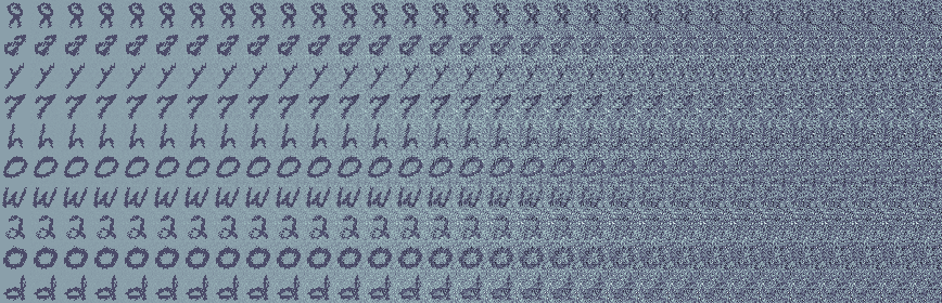
Diffusion models have made quite a splash, especially after the open-source release of Stable Diffusion. What are diffusion models, where does the loss come from and what does a simple example look like? I've recently helped open-source a simple, pedagogical, self-contained example colab of a diffusion model trained on EMNIST, which you can find as part of the Variational Diffusion Models (VDM) github page. In this post, I wanted to give some more background and a simple way to motivate where the loss function comes from.

Non-negativity of KL

Let's say we want to build a latent-variable model, $𝑞 (𝑥, 𝑧)$ where the likelihood of the data ( $𝑝 (𝑥)$ ), has high marginal likelihood: $l o g 𝑞 (𝑥)$ . Unfortunately, computing $l o g 𝑞 (𝑥)$ involves an intractable integral over the latent variable, $𝑧$ .¹

³ I use brakets to show expectations and unless noted, always with respect to the full

𝑝

distribution.

⟨ \cdot ⟩ 𝑝 = 𝔼 𝑝 [\cdot] = \int 𝑑 𝑥 𝑝 (𝑥) [\cdot]

If I don't denote the distribution the expectation is with respect to on the brakets, it's always the full joint $𝑝 (𝑥, \dots)$ . Notice that this works even if there are fewer variables or conditioning variables left inside the terms in the brakets, as any excess variables will just marginalize out without issue in the expectation and any variables being conditioned on will be evaluated in expectation as desired.

We can derive the tractable objective used to train these models using the observation that the KL² divergence is non-negative and monotonic. The Kullback-Leibler (KL) divergence between any two distributions is non-negative:³ $⟨ l o g 𝑝 (𝑥) 𝑞 (𝑥) ⟩ 𝑝 \geq 0 .$

If we marginalize out some subset of random variables the KL divergence of the marginal distributions has to be less. For any two random variables: $⟨ l o g 𝑝 (𝑥, 𝑧) 𝑞 (𝑥, 𝑧) ⟩ = ⟨ l o g 𝑝 (𝑥) 𝑝 (𝑧 | 𝑥) 𝑞 (𝑥) 𝑞 (𝑧 | 𝑥) ⟩ = ⟨ l o g 𝑝 (𝑥) 𝑞 (𝑥) ⟩ + ⟨ l o g 𝑝 (𝑧 | 𝑥) 𝑞 (𝑧 | 𝑥) ⟩ \geq ⟨ l o g 𝑝 (𝑥) 𝑞 (𝑥) ⟩ \geq 0$ Intuitively, if we think about KL divergence as a "distance" between probability distributions, two joint distributions always have to be at least as far apart as their marginals. As we just saw, the KL of the joint is the sum of the KL between the two marginals, as well as the expected KL of the conditional distributions (which has to be positive, as all KLs are).

VAEs

Imagine designing these joint distributions to have different flavors. Think of $𝑝 (𝑥, 𝑧)$ as a forward process $𝑝 (𝑥) 𝑝 (𝑧 | 𝑥)$ that takes an image from some natural image distribution $𝑝 (𝑥)$ and then encodes it into some representation $𝑧$ with an encoder $𝑝 (𝑧 | 𝑥)$ . This is a joint distribution over the two variables. Running the forward process would give us $(𝑥, 𝑧)$ pairs, pairs of natural images and their encodings. Next, imagine a different joint distribution, a reverse process $𝑞 (𝑥, 𝑧)$ that takes some sample from a prior $𝑞 (𝑧)$ and then runs it through a decoder $𝑞 (𝑥 | 𝑧)$ to generate a synthetic image. This is a generative model of the kind we might be used to building. This is also a fully-fledged joint distribution that we could sample from, in order to generate $(𝑥, 𝑧)$ pairs. At initialization, these two distributions are very different. The goal of generative modeling is to bring these two joint distributions into alignment.

Based on the properties of the KL divergence, these two joint distributions must have a non-negative KL divergence that is monotonic to marginalizing out one of the variables: $⟨ l o g 𝑝 (𝑥, 𝑧) 𝑞 (𝑥, 𝑧) ⟩ = ⟨ l o g 𝑝 (𝑥) 𝑝 (𝑧 | 𝑥) 𝑞 (𝑧) 𝑞 (𝑥 | 𝑧) ⟩ \geq ⟨ l o g 𝑝 (𝑥) 𝑞 (𝑥) ⟩ \geq 0$ Notice what this is saying. The KL divergence between the joint distributions here is the expected log density ratio of the forward to the reverse model's likelihood, where the expectation -- the samples -- are taken with respect to the forward process $𝑝 (𝑥, 𝑧)$ . This joint KL is itself an upper bound for the KL divergence between the marginal distributions $𝑝 (𝑥)$ and $𝑞 (𝑥)$ . $𝑝 (𝑥)$ was our original image distribution, while $𝑞 (𝑥)$ is the distribution of synthetic images drawn from the generative model that is our reverse process: $𝑞 (𝑥) = \int 𝑑 𝑧 𝑞 (𝑥 | 𝑧) 𝑞 (𝑧)$

So, by minimizing the KL between our forward and reverse process -- by aligning the two joint distributions -- we can ensure that we make progress towards learning a good generative model of our images $𝑞 (𝑥)$ . We can ensure that we are aligning the marginals $𝑞 (𝑥)$ and $𝑝 (𝑥)$ .

The tightness of this bound is controlled by how close together the remaining conditional distributions are:

$⟨ l o g 𝑝 (𝑥, 𝑧) 𝑞 (𝑥, 𝑧) ⟩ = ⟨ l o g 𝑝 (𝑥) 𝑞 (𝑥) ⟩ + ⟨ l o g 𝑝 (𝑧 | 𝑥) 𝑞 (𝑧 | 𝑥) ⟩$ In other words: the degree to which our encoding distribution ( $𝑝 (𝑧 | 𝑥)$ ) matches the Bayesian posterior of our generative model ( $𝑞 (𝑧 | 𝑥)$ ) determies the tightness of our bound.

So, again, all we started with is the idea of two different processes, the forward process that takes images and encodes them and a reverse process that samples some latents from a known distribution and decodes them. If we try to minimize the KL divergence between these two processes, forward to reverse, we can ensure that this is a valid bound on the marginal KL between the true image distribution $𝑝 (𝑥)$ and the marginal of our generative model $𝑞 (𝑥)$ . That is, by learning to make the two joint processes look alike we are also as a consequence learning a good generative model of images.

We've just derived the ordinary ELBO:⁴

⟨ l o g 𝑝 (𝑥, 𝑧) 𝑞 (𝑥, 𝑧) ⟩ = ⟨ l o g 𝑝 (𝑥) - l o g 𝑞 (𝑥 | 𝑧) + l o g 𝑝 (𝑧 | 𝑥) 𝑞 (𝑧) ⟩,

up to a constant outside our control, the entropy of the true image distribution

𝑝 (𝑥)

. Notice that this term cancels out on both sides if we wish to target the cross-entropy from our true

𝑝 (𝑥)

to our model's

𝑞 (𝑥)

rather than the KL.

$⟨ l o g 𝑝 (𝑥, 𝑧) 𝑞 (𝑥, 𝑧) ⟩ = ⟨ l o g 𝑝 (𝑥) - l o g 𝑞 (𝑥 | 𝑧) + l o g 𝑝 (𝑧 | 𝑥) 𝑞 (𝑧) ⟩ \geq ⟨ l o g 𝑝 (𝑥) 𝑞 (𝑥) ⟩ ⟨ - l o g 𝑞 (𝑥 | 𝑧) + l o g 𝑝 (𝑧 | 𝑥) 𝑞 (𝑧) ⟩ \geq ⟨ - l o g 𝑞 (𝑥) ⟩ ⟨ l o g 𝑞 (𝑥) ⟩ \geq ⟨ l o g 𝑞 (𝑥 | 𝑧) - l o g 𝑝 (𝑧 | 𝑥) 𝑞 (𝑧) ⟩$

At the end of the day, the hope and the dream we seem to have in doing latent variable modeling is that maybe we will somehow be more successful in learning a reverse $𝑞 (𝑧) 𝑞 (𝑥 | 𝑧)$ process to match some forward $𝑝 (𝑥) 𝑝 (𝑧 | 𝑥)$ than we would have been able to just model the density $𝑞 (𝑥)$ directly. We are hoping that by expanding the problem, and making it a harder or larger modeling task, it'll become easier for us to optimize or learn.

Diffusion

For diffusion models, honestly, there isn't much to add except they add many more steps. The only difference is that instead of a two-step forward process, in diffusion we imagine a many-stepped (or potentially continuous) forward and reverse process.

In particular, in most diffusion models we fix the forward process to be a Markov chain: $𝑝 (𝑥, 𝑧 0, 𝑧 1, 𝑧 2, \dots, 𝑧 𝑇 - 1, 𝑧 𝑇) = 𝑝 (𝑥) 𝑝 (𝑧 0 | 𝑥) 𝑝 (𝑧 1 | 𝑧 0) \dots 𝑝 (𝑧 𝑇 | 𝑧 𝑇 - 1),$ which starts with a sample from a natural image distribution $𝑝 (𝑥)$ and then adds $𝑇$ steps of additive Gaussian noise $𝑝 (𝑧 𝑡 | 𝑧 𝑡 - 1) \sim N (𝛼 𝑡 𝑧 𝑡 - 1, 𝜎 2 𝑡)$ .

Graphical model showing the forward process for diffusion. — Figure 1. The graphical model for the forward process in diffusion.

This takes an ordinary image and then adds more and more noise to it until it looks more or less indistinguishable from just isotropic Gaussian noise.⁵

Illustration of standard forward diffusion process as additive Gaussian noise. — Figure 2. A demonstration of the typical forward process in diffusion models.

One particularly nice thing about using Gaussians for every step of the forward process here is that the composition of a bunch of conditional Gaussians is itself Gaussian so we will have a closed form for the marginal distribution at any intermediate time: $𝑝 (𝑧 𝑡 | 𝑥) = N (˜ 𝛼 𝑡 𝑥, ˜ 𝜎 2 𝑡 𝐼) .$

With a forward process defined, we parameterize or learn the reverse process, a Markov chain that operates in the opposite direction: $𝑞 (𝑥, 𝑧 0, 𝑧 1, \dots, 𝑧 𝑇) = 𝑞 (𝑧 𝑇) 𝑞 (𝑧 𝑇 - 1 | 𝑧 𝑇) \dots 𝑞 (𝑧 1 | 𝑧 2) 𝑞 (𝑧 0 | 𝑧 1) 𝑞 (𝑥 | 𝑧 0)$

Graphical model showing the reverse process for diffusion. — Figure 3. The graphical model for the reverse process in diffusion.

The VDM loss is⁶ simply the KL between these two joints, which serves as an upper bound on the KL of the image marginals: $⟨ l o g 𝑝 (𝑥, 𝑧 0, 𝑧 1, \dots, 𝑧 𝑇) 𝑞 (𝑥, 𝑧 0, 𝑧 1, \dots, 𝑧 𝑇) ⟩ \geq ⟨ l o g 𝑝 (𝑥) 𝑞 (𝑥) ⟩$

Just as in the case of a VAE, here, the hope is that it might actually be easier to model the larger joint distribution than it was to try to model the density directly. In the case of simple diffusion models, the forward process is fixed additive Gaussian noise. If we make enough steps in the forward process we believe we ought to be able to learn the reverse process exactly.⁷

Various Sundry Tricks

The joint KL is equivalent to the VDM loss. However, in practice, to make this loss efficient to train, diffusion models leverage a lot of the known structure of the forward process to power a very clever parameterization of the reverse process. This requires some tricky rearranging of terms and some stochastic approximation to make the whole thing efficient.
To see the code, please check out the example colab as well as its accompanying text that walks through some of these details in more detail.

To utilize our knowledge of the forward process, we're actually going to rewrite the forward process not as a sequence of conditional Gaussian steps (a bottom-up forward process): $𝑝 (𝑥, 𝑧 0, 𝑧 1, 𝑧 2, \dots, 𝑧 𝑇) = 𝑝 (𝑥) 𝑝 (𝑧 0 | 𝑥) 𝑝 (𝑧 1 | 𝑧 0) 𝑝 (𝑧 2 | 𝑧 1) \dots 𝑝 (𝑧 𝑇 | 𝑧 𝑇 - 1)$ but instead we'll rearrange this to be a product of a bunch of conditional reverse steps (as a top-down forward process): $𝑝 (𝑥, 𝑧 0, 𝑧 1, 𝑧 2, \dots, 𝑧 𝑁) = 𝑝 (𝑧 0, 𝑧 1, 𝑧 2, \dots, 𝑧 𝑇 | 𝑥) 𝑝 (𝑥) = 𝑝 (𝑧 0 | 𝑧 1, \dots, 𝑧 𝑇, 𝑥) 𝑝 (𝑧 1 | 𝑧 2, \dots, 𝑧 𝑇, 𝑥) \dots 𝑝 (𝑧 𝑇 | 𝑥) 𝑝 (𝑥) = 𝑝 (𝑧 0 | 𝑧 1, 𝑥) 𝑝 (𝑧 1 | 𝑧 2, 𝑥) \dots 𝑝 (𝑧 𝑇 - 1 | 𝑧 𝑇, 𝑥) 𝑝 (𝑧 𝑇 | 𝑥) 𝑝 (𝑥)$ For the Gaussian diffusion, we can analytically figure out what these conditional reverse steps should be for the forward process $𝑝 (𝑧 𝑡 - 1 | 𝑧 𝑡, 𝑥)$ . These distributions compute the probability of seeing a particular noisy image from the previous step if we get to observe both the noisy image as well as the original image.

Graphical model showing the top-down generative process for diffusion. — Figure 4. The graphical model for the top-down forward process in diffusion.

We'll then parameterize our reverse process $𝑞 (𝑧 𝑡 - 1 | 𝑧 𝑡)$ to have this same functional form: $𝑞 (𝑧 𝑡 - 1 | 𝑧 𝑡) \leftarrow 𝑝 (𝑧 𝑡 - 1 | 𝑧 𝑡, ˆ 𝑥 (𝑧 𝑡, 𝑡)) .$ We'll model the reverse process as if it were the exact reversed conditional forward process, but of course, for the true reverse process we don't get to observe the true original image. Still, we'll use the same functional form, it's just we'll spend our modeling budget on trying to impute the original clean image $ˆ 𝑥$ after observing the noisy image $𝑧 𝑡$ and which step we are on $𝑡$ .

The actual parametric model in a diffusion model is this bit, $ˆ 𝑥 (𝑧 𝑡, 𝑡)$ . It is a neural network that takes as input the noisy image $𝑧 𝑡$ and the step we are on in the diffusion process $𝑡$ and has the job of trying to predict what the corresponding clean image was that generated the noisy image. In most diffusion models this is implemented as a U-Net style architecture. In practice, it's been found that if instead of predicting the clean image $ˆ 𝑥$ , you predict the noise $ˆ 𝜖$ from the noisy image, you get better-looking samples.⁸ The full reverse generative model then consists of many steps of looking at a noisy image and trying to infer the clean one; rinse and repeat.

With these choices in place, we can now look at the full joint KL and organize terms.

$⟨ l o g 𝑝 (𝑥) - l o g 𝑞 (𝑥 | 𝑧 0) + l o g 𝑝 (𝑧 𝑇 | 𝑥) 𝑞 (𝑧 𝑇) + 𝑇 - 1 \sum 𝑖 = 0 l o g 𝑝 (𝑧 𝑖 | 𝑧 𝑖 + 1, 𝑥) 𝑞 (𝑧 𝑖 | 𝑧 𝑖 + 1) ⟩ 𝑝$

The last trick we're going to use is that we're going to avoid computing all of the terms in our sum by simply not computing all of the terms in our sum. We'll approximate the sum with Monte Carlo: we'll simply randomly choose one of the terms and upweight it appropriately. At that point, we have the loss function used to train VDM models. A very nice thing about the VDM loss is that it is clear that we are optimizing a bound on the marginal likelihood of our generative model. As you can learn in the VDM Paper, many of the diffusion models you've heard about correspond to a weighted form of this same objective, where different terms in the sum get different weights.

After going through all of the fancy math, the analytic KL divergences involved in the diffusion loss simplify quite nicely: $⟨ l o g 𝑝 (𝑥) - l o g 𝑞 (𝑥 | 𝑧 0) + l o g 𝑝 (𝑧 𝑇 | 𝑥) 𝑞 (𝑧 𝑇) + 12 𝑇 - 1 \sum 𝑡 = 0 𝛽 𝑡 ∥ 𝜖 - ˆ 𝜖 (𝑧 𝑡, 𝑡) ∥ 2 ⟩$ For variational diffusion the weight terms $𝛽 𝑡$ depend on your choice of noise schedule. For most other diffusion models in the wild, these $𝛽 𝑡$ weights are conventionally set to 1.

Closing Thoughts

So, why are diffusion models so interesting? Well, first and foremost, the reason they are drawing so much attention is that they have shown tremendous performance. It feels like for the first time we have models that are able to generate very high resolution, very high fidelity natural images. Projects like DALL-E2, Imagen, and Stable Diffusion show really impressive results. What is the magic driving these models?

At a high level, I think we can say that diffusion models start to realize the dream of latent variable models. Sometimes, when you are faced with a problem that is too difficult, you can crack it if you consider an even harder, related problem. As I tried to demonstrate here, even for simple latent variable models like VAEs and especially for diffusion models, one reason we can point to for their success is that instead of directly modeling the distribution over images, they model a much larger joint distribution. That larger joint distribution is strictly speaking a bigger thing to attempt to model, but here we get to design the forward process in such a way that even if there are many pieces to the forward process, those pieces individually are easier to tackle.

However, if that were the case, shouldn't we have expected deep hierarchical models to perform similarly awesomely? Probably, though here I think there is another real trick that diffusion has up its sleeve. For a general deep hierarchical generative model, even if by splitting the problem up into smaller pieces you might have split it up into easier-to-model tasks, to evaluate the joint KL you still need to evaluate all of those terms. That is, as your model becomes richer and more computationally expressive because of its depth, so does the cost of training your model, as you have to evaluate all of the layers at each step in the training process.

Diffusion models avoid this by structuring their forward process in such a way that all of the steps share a great deal of structural similarity. This allows diffusion to approximate a sum of a potentially large number of steps by a single randomly chosen step. If each step looks more or less the same, you can get a good estimate for the whole sum by looking at an individual, random, term.

The last trick up its sleeve is, even if you managed to design a deep hierarchical generative model with this structural homogeneity property, if you wanted to get to some intermediate position in the hierarchy you'd still have to run roughly half of the full forward process. That would still be expensive in general. Here, diffusion avoids that entirely.
As boring as a sequence of conditional Gaussians is as a forward process, it is also beautiful: it enables exact analytic marginalization to intermediate steps. You can very quickly mimic the result of adding hundreds of steps of additive Gaussian noise by simply adding a moderate amount of Gaussian noise in a single shot.

So, ultimately, what do I think is one of the main reasons diffusion models do so well? I think it's because they can do so well! I think it's because they are very powerful, expressive, generative models. Sampling from them is generally rather expensive. Drawing a sample means running the full reverse process, which might mean calling the central score net a thousand or so times. That is a very powerful and very expressive generative model, but magically, we can train that generative model's likelihood without ever having to actually instantiate the full generative process at training time due to our set of sundry tricks.

I'm excited to see where this all goes and hope this post and the colab help to introduce these magical models to a wider audience.

Special thanks to Ben Poole, Pavel Izmailov, Christopher Suter, and Sergey Ioffe, and Ian Fischer for helpful feedback on this post.